How to Simulate a Ponytail

Or, Lagrange Multiplier Constrained Rigid Body Dynamics

If you're writing your own rigid body physics simulator, after you've got the bodies bouncing around as independent 6 degrees of freedom (DOF) objects, and interacting with springs, damping, gravity, and other external forces, and you've added single-point collisions between the bodies and the world, what's next?

Two useful next steps are to add support for resting contact so the bodies can stack, and to add hard constraints so you can build more interesting compound jointed mechanisms, like ragdolls and cars and whatnot. Resting contact is in some ways a superset of hard constraints, and it's certainly more difficult to do right, so a good next step in learning is to implement constraints.

There are a lot of ways to implement hard constraints, and they vary in performance, stability, accuracy, and difficulty of programming. They each have pros and cons. Some of the more popular methods include:

• Augmented Coordinates / Lagrange Multipliers with explicit integration
  • The topic of this article.
• Generalized Coordinates and explicit integration
  • Often Featherstone's and Balafoutis and Patel's algorithms are used for this, also see my Physics References.
• Implicit integration with springs/potentials and/or generalized coordinates
  • Dave Wu is the master of this, and I've implemented several variations based on his research.
• Iterative projection based fixup methods
  • Thomas Jakobsen's excellent GDC presentation discusses this method.

I've implemented all of these and a few others to boot (see Five Physics Simulators for Articulated Bodies for discussion of the first three as well), and I hope to eventually have articles about all of them, and discuss the tradeoffs and pros and cons.

Lagrange Multipliers

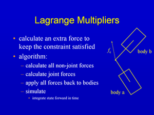
The first technique I implemented when I was investigating constrained dynamics were "Augmented Coordinates with Lagrange Multipliers". It sounds complicated, but at its heart it simply means you calculate all the known external forces on your objects from things like gravity, springs, explosions, and whatnot, and then you compute the forces necessary to add into those external forces to keep the constraints satisfied. So, if you have an object constrained to slide on the floor, and you're not pulling on it, the constraint forces computed might be 0, or they might be just enough to counteract gravity if you're simulating it. If you pull up, the constraints pull down to cancel out your pull. If you slide the block sideways, the constraint forces do not try to stop you, and the block slides, but can't move up and down.

In that example, we were probably using a 3DOF constraint, one translational DOF to prevent the block from leaving the floor, and 2 rotational DOFs to prevent the block from rotating except about the normal to the floor (so it doesn't rotate into the floor). One great feature of Lagrange Multiplier constraints is that they explicitly subtract off the DOFs one at a time, and you can control them in a very modular way. So, you can easily have the same code handle constraining any combination of the 6 DOFs of a rigid body. Once you get your simulator working (or if you play with my sample code below) you can see this modularity in action.

The Math

The math for Lagrange Multiplier constraints is very clean and elegant, and it can be expressed at a high level very parsimoniously. Here is the full general derivation of the technique for arbitrary DOF constraints. Obviously, the lecture and articles below go through this math at a much lower level and with more details, and they don't actually lift up to this level of generality due to space and time constraints, but all the detailed nitty gritty math in the lecture and articles is subsumed by this math in its most general form. It is worth noting the sample code actually does directly implement this general math, however.

Constrained Dynamics in 4 Easy Steps
Start out with the matrix version of Newton's f=ma, with explicit known external forces, fe, and unknown constraint forces, fc.		$\mathbf {M{\ddot {q}}=f_{e}+f_{c}}$	(1)
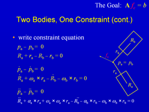
Form the constraint equations for the state vector q, and differentiate them twice.		${\begin{array}{lclcr}\mathbf {C(q)} &=&&&\mathbf {0} \\\mathbf {{\dot {C}}(q)} &=&\mathbf {J{\dot {q}}} &=&\mathbf {0} \\\mathbf {{\ddot {C}}(q)} &=&\mathbf {J{\ddot {q}}+{\dot {J}}{\dot {q}}} &=&\mathbf {0} \end{array}}$	(2)
Symbolically solve for the accelerations (M is trivially invertible because these are augmented coordinates) in terms of the workless constraint forces, using the Jacobian transpose and λ as the unknown Lagrange multipliers.		${\begin{array}{lcl}\mathbf {\ddot {q}} &=&\mathbf {M^{-1}(f_{e}+f_{c})} \\&=&\mathbf {M^{-1}(f_{e}+J^{T}{\boldsymbol {\lambda }})} \end{array}}$	(3)
Form an Ax=b matrix equation for the unknonwn λ multipliers, solve for them, then substitute them back into (3) to find the accelerations.		${\begin{array}{rcl}\mathbf {JM^{-1}J^{T}{\boldsymbol {\lambda }}} &=&\mathbf {-{\dot {J}}{\dot {q}}-JM^{-1}f_{e}} \\\mathbf {A{\boldsymbol {\lambda }}} &=&\mathbf {b} \end{array}}$	(4)

Writing Constraint Equations

After you've got the basic constraint structure in place, it all comes down to writing the constraint equations. The articles, lecture, and sample code all just focus on a 3DOF point constraint, but I'll eventually write up some stuff about implementing other kinds of constraints. Writing constraint equations is actually a deeper exercise than it appears initially, there is some really important math to explore in writing the signed distance functions that make good constraint equations.

todo: lots more work to do on this page

Lectures and Articles

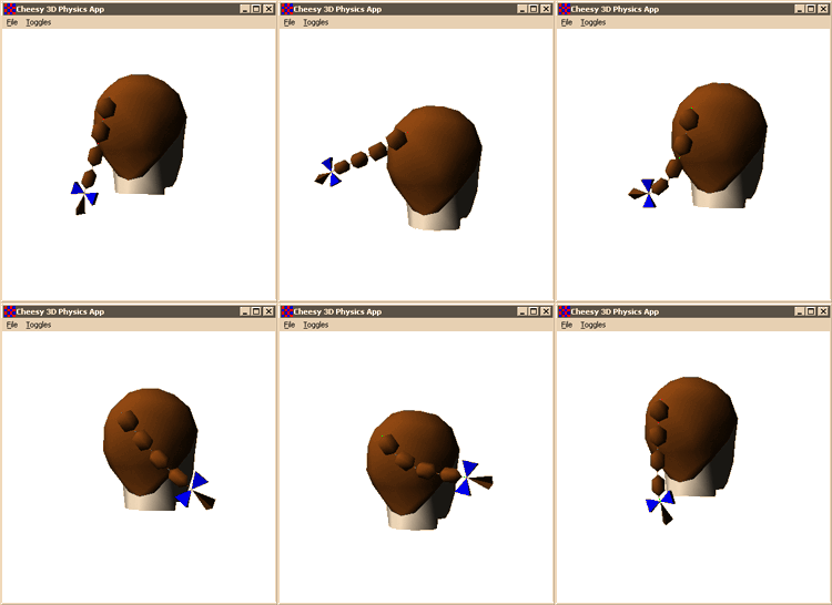
I decided to extend my rigid body articles to discuss simulating a ponytail with hard constraints back in 1999 at the Game Developers Conference Roadshow in Seattle, then I wrote a two-part article about it for Game Developer Magazine and gave the lecture at the 2000 GDC.

The materials...

• How to Simulate a Ponytail, the lecture slides. I think I have an old audio tape of this lecture somewhere, and if I ever find it I'll convert it to an mp3 and post it here. I think this was the best hardcore math lecture I ever gave. It was completely step-by-step and explicit, and the entire goal was to derive a Lagrange Multiplier constraint solver, and it moved fast, but not too fast, and it was crystal clear by the end how each chunk worked. Or, at least, I thought so!  :) If anybody else has the audio tape of this, please send me mail.

• How to Simulate a Ponytail, the articles: Part 1 and Part 2. These are basically the same as the lecture but in article format, which has advantages and disadvantages.

• How to Simulate a Ponytail, the sample code, zipped. This is a very straightforward (read: inefficient) implementation of Lagrange Multiplier constraints. It only implements point constraints, but the core of the simulator is super general, so you could trivially try out different kinds of constraints with this code. It copies large matrices around all over the place, but computers are fast and its implementation directly mirrors the mathematical derivation mentioned above. You need a C++ compiler to build this code, and it uses OpenGL and either Win32 or GLUT.